The Design of Bilateral Routing Algorithm Given the Utility Parameter from the Road User View
Ali Hatefi1 * , Mohammad Omidvar1 and Mohammadreza Noabadi1
1
Technical and Vocational Training College,
Islamic Azad University,
Mashhad Branch,
Mashhad
Iran
http://dx.doi.org/10.12944/CWE.10.Special-Issue1.72
In this study, a new approach in the design of routing algorithm to start from the origin and destination and its situation is designed. In this algorithm utility parameter from the road user view that the path as possible is short and straight is considered. One of the outputs of this algorithm is provide the balance curve of path costs. using the balance curve of path costs will be design based on the available budget and available funds, the optimal path.
Copy the following to cite this article:
Hatefi A, Omidvar M, Noabadi M. The Design of Bilateral Routing Algorithm Given the Utility Parameter from the Road User View. Special Issue of Curr World Environ 2015;10(Special Issue May 2015). DOI:http://dx.doi.org/10.12944/CWE.10.Special-Issue1.72
Copy the following to cite this URL:
Hatefi A, Omidvar M, Noabadi M. The Design of Bilateral Routing Algorithm Given the Utility Parameter from the Road User View. Special Issue of Curr World Environ 2015;10(Special Issue May 2015). Available from: http://www.cwejournal.org/?p=9407
Download article (pdf)
Citation Manager
Publish History
Introduction
The roads are considering one of the national capitals of the country; as yet several researches concerning routing with low cost is applied. As much as possible design with the limited budget available. The ideal way to shorten the path, is based on the lowest cost. The costs can include environmental costs, the cost of land ownership, the cost of road construction, road user and maintenance, the various studies has been done on quantifying the cost parameters (Hatefi, 2006). Since the aim of this study was design of routing algorithms based on cost parameters are listed, hypothetically network considered for the analysis of the results and the algorithm has been implemented on a given network.
A Review of Past Research
The Most of the articles published in the algorithm is the fastest route with static networks. Networks with a fixed topology and costs are fixed through an average traveling time would be best. In this study, unlike conventional methods of raster GIS network use. The raster GIS network is capable of processing and network analysis is less known. There is various software functions are raster analysis. It began in 1736 when Euler's famous question posed Konigsberg bridge. The problem was that after a certain point in the city to find a way each of the Seven Bridges of Konigsberg is a historically notable problem in mathematics. Its negative resolution by Leonhard Euler in 1735 laid the foundations of graph theory and prefigured the idea of topology.
In 1979, Pang & Dew the list of algorithms for the fastest way is set (Husdal, 2000).the list more than 222 different routing algorithms have been developed in the 1958. They have an excellent research and a brief description of each category of algorithms and a comparison between specific algorithms is embodied. Some of these methods to routing are static networks with specific cost pass Is dedicated.
Several algorithms were developed with different data structure so that in 1959 Dijkstra's algorithm was invented (Dijkstra, 1959). Dijkstra's algorithm, conceived by computer scientist Edsger Dijkstra is a graph search algorithm that solves the single-source shortest path problem for a graph with non-negative edge path costs, producing a shortest path tree. This algorithm is often used in routing and as a subroutine in other graph algorithms.
For a given source vertex in the graph, the algorithm finds the path with lowest cost (i.e. the shortest path) between that vertex and every other vertex. It can also be used for finding costs of shortest paths from a single vertex to a single destination vertex by stopping the algorithm once the shortest path to the destination vertex has been determined. For example, if the vertices of the graph represent cities and edge path costs represent driving distances between pairs of cities connected by a direct road, Dijkstra's algorithm can be used to find the shortest route between one city and all other cities.
In 1995 in order to the zigzag motion improvement in coverage area of an effort was carried by Xu and Lathrop (Xu et al., 1995). According Xu and Lathrop cumulative cost of non-adjacent cells, each cell x to y as the total cumulative costs of each of the cells in the direction of x to y in the geometric distance is measured. McIlhagga new words as "cost - fixed distance" introduced.
McIlhagga (McIlhagga, 1997) algorithm development of Ron Eastman method. This algorithm is used when you have multiple targets. In other words, the algorithm is cost optimal level if all targets in the path consider is found. The pillar view from the coincident on least-cost path is also interesting. The idea is based only on networks at the least expensive route to take action is not, the idea is the cost through a steep slope and connects , so this idea of the cost of a route on a steep slope know more than the cost of passing on a steep slope (Collischonn et al., 2000). Their algorithm for determining the net cost is the cost - slope function. The output of this algorithm is not a straight line on a mountain path and go up the mountain rounder.
Barry uses a concept similar to the concept Tomlin (Berry, 2000). He called this algorithm splash, Splash algorithm to create a surface displacement of the 8 adjacent cells to be used anywhere else. Cumulative distance and relative costs are estimated for each of the 8 possible steps. The Step in the overall cost to the displacement. Then the optimal path from any point of origin as the sharpest slide on the specified level (the same channel on the mountain). To find the optimal path between two points Barry suggest go to both the cumulative cost to create add together these points.
Barry also invented the concept of routing between multiple points. He called the practice of cumulative step. The path between point 1 and point 2 is then calculated between point 2 and point 3 is calculated route. This process is repeated for each other along the way, although this method is not the best option for areas located along the path, but its advantage is that for them in the order in which they appear on the path we've taken the work that is done in the calculation of all possible combinations of levels of aggregation step and choose the best combination of them. This concept can be used to calculate the optimal route in successive intervals.
Cost Level
According to the definition of cost level is the map where each cell show cost pass of the cell Cost Levels symmetric and asymmetric are made (Eastman, 1997).
Convert One Level to Network
In raster GIS defined intervals on the surface so that the value of a specific attribute on the surface may vary. For communication and processing network structure of each cell should be considered as a node. The representative of the cost of each node cells from these cells. Each of these values are considered as the weight of the cell has a minimum cost path to find them. The weights as resistance or friction or difficulty passing through these values can be considered the most - cost-interval considered.
The Calculation begins of certain destination and extends to the surrounding and adjacent to each of the cells through the cell adjacent to the cumulative total cost is calculated according to the cumulative cost of a minimum cost path from each cell to the destination is obtained (Douglas, 1994). The disadvantages of the method was initially delivered straight lines (horizontal or vertical) were defined on the Network and obtained path would be a zig-zag path.
A-Star Algorithm to Find the Shortest Path
The fundamental equation that determines whether each of the cells have the privilege to be in the following form:
F = G + H (1)
Where G is a function of distance from the origin is based on Dijkstra's algorithm and H distance estimate to the destination for each cell. Estimates of H downstream lead to slowing the progress of the processing algorithms to increase the processed range. If H is an estimate of the upstream remaining path, one of these methods is the Manhattan distance. The distance between two points in a grid based on a strictly horizontal and/or vertical path (that is, along the grid lines), as opposed to the diagonal or "as the crow flies" distance. The Manhattan distance is the simple sum of the horizontal and vertical components. The disadvantage of this method is that it is not very much in line with the method of measuring g parameter.
Implementation
Path Utility Parameter
From a user perspective the most optimal path between two points is a straight line. To apply the parameters of the utility of this study, a total distance of the center of each cell of origin and destination, multiplied by the cost of its acquisition, the cell will cost alternative. This method is also considered utility path. For example, in Figure 1, two points p and q have the same utility. Because of the point total of 7 units of distance p and q point total of 10 units and 14 units of distance, cost and unit cost is 5, so both are the utility 70.
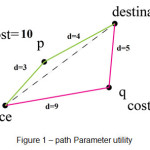 |
Figure 1: path Parameter utility Click here to View figure |
As the diagram in Figure 2 shows, the utility of each cell (U) by multiplying the cost of ownership of the cell (C) The total distance from the cell of origin (d1) and destination (d2) can be obtained by:

The Method Used to Calculate G
G is calculated based on distance from the origin cell and Dijkstra's algorithm calculated as follows:

In relation (3), gi represents the cost of the path to my cell i, Ui, indicating the utility of cell i is the i-th and j-th cell is the distance dij
The Method Used to Estimate H
First, each cell as the source and the destination cell algorithm that calculates the cost. Dijkstra's Secondly the cost destination to the selected cell is calculated based on the Dijkstra's algorithm. Comparison of two methods of the first and second H is at least as selective in terms of the function F is considered.
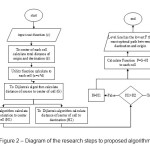 |
Figure 2: Diagram of the research steps to proposed algorithm Click here to View figure |
The Shortest Path Algorithm
As the diagram in Figure 2 shows, in the first stage cost function is defined for all cells. Cost per cell can be quantitative or qualitative outcome costs, all of which are a little figure has been calculated and recorded. Then the function F, G and H are calculated and the results are determined. The algorithm is based on Dijkstra's algorithm, once cost to the target cell and the cell once the target cost is calculated as the minimum value between the value of the parameter H to provide. Figure 3 is a picture of the various stages of implementation of the algorithm on the given data is shown.
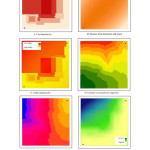 |
Figure 3: The various steps of implementation of the proposed algorithm is based on the assumption Click here to View figure |
Implementation and Testing of Algorithms
To implement this algorithm to a hypothetical network used 50 x 50 that cell dimensions 1*1 meter is intended. The procedure for the Python programming language is used. The final output of this algorithm is a function F whose value represents the cost for each cell through the cell path between origin and destination Figure 4 compares the results of the implementation of the results of the algorithm shows. As shown in Figure 4-c , the proposed route is determined by considering the utility parameter from a user view would be some path to the center.
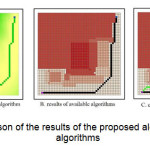 |
Figure 4: Comparison of the results of the proposed algorithm and available algorithms Click here to View figure |
Discussion
The new algorithm is able to achieve the level curve path cost, Therefore, we can design the optimal route based on the available budget and there is as possible add buffer the utility function it means the utility can also be considered as a point. For example, if a particular group or organization is willing to invest in the road, can be effect the amount of capital to buffer to the new route was designed. The algorithm can be set up to answer that could be a set of answers with regard to the amount of capitals available to be accessed. The most performance of the algorithm for creating level curve paths cost is between origin and destination.
Suggestions
- Development of algorithms for the design of multi-destination & origin routing algorithm
- Integrate this algorithm with pso algorithm and compare its results
- Integrate the proposed algorithm to genetic algorithm and compare its results
- Work on simplification algorithm in long path
Acknowledgement
This paper is based on work supported by the technical and vocational training college, Islamic Azad University, Mashhad Branch, Mashhad. any opinions, findings, and conclusions or recommendations exposed proposed in this paper are those of authors and do not necessarily reflect those of technical and vocational training college, Islamic Azad University, Mashhad Branch, Mashhad.
References
- Berry, J. Analyzing accumulation surfaces, Map Analysis: Procedures and Applications in GIS Modeling. Berry and Associates//Spatial Information Systems Inc. (2000).
- Collischonn, W., & Pilar, J. V. A direction dependent least-cost-path algorithm for roads and canals. International Journal of Geographical Information Science, 14(4), 397-406 (2000).
- Dijkstra, E. W. A note on two problems in connexion with graphs. Numerische mathematik, 1(1), 269-271 (1959).
- Douglas, D. H. Least-cost path in GIS using an accumulated cost surface and slopelines. Cartographica: the international journal for Geographic Information and Geovisualization, 31(3), 37-51 (1994).
- Eastman, R. Idrisi for Windows User’s Guide (Worcester, MA, USA: Clark University) (1997).
- Hatefi, A. Pathfinding with respect to iteration process and gis. university of ferdovsi mashhad, Iran (2006).
- Husdal, J. An investigation into fastest path problems in dynamic transportation networks. Unpublished, coursework for the M. Sc. in GIS, University of Leicester. (2000).
- McIlhagga, D. Optimal path delineation to multiple targets incorporating fixed cost distance. Unpublished Thesis, Carleton University, Ottawa, ON. (1997).
- Xu, J., & Lathrop Jr, R. G. Improving simulation accuracy of spread phenomena in a raster-based geographic information system. International Journal of Geographical Information Systems, 9(2), 153-168 (1995).